|
Summary
The retrieval of δD vertical profiles from IASI spectra described here corresponds to the retrieval developed at
ULB/LATMOS. We provide daily
retrievals of δD in the tropics corresponding to the morning orbit of IASI (no evening orbit). IASI δD vertical profiles have limited
vertical information with degrees of freedom between 1.5 and 2 indicating between 1 and 2 independent levels of
information with a coarse vertical resolution (3 km). The maximum of sensitivity generally lies in the free troposphere
between 3 and 6 km and part of the information can also come from the boundary layer. There is no information at the surface,
except in particular case of high thermal contrast between the surface and the first layer of the atmosphere.
Because of the limited vertical sensitivity, the user must consider the averaging kernels of the retrieval in the analysis
of IASI δD data. Wiegele et al., 2014 suggest to apply an a posteriori correction on joint humidity and δD retrieved profiles in order to
ensure they are representative of the exact same vertical layer of the atmosphere.
|
Each file contains, for one day of observation, level-2 HDO and H2O profiles for the tropics (30S-30N) and for the AM orbit.
File names include date of observation. Their structure is :
SENSOR_PLATFORM_LEVEL_"HDO"_YYYYMMDD_"ATMOSPHIT"_VERSION_"AM_TROPICS.nc"
where : SENSOR = IASI, PLATFORM = metopa, LEVEL = L2, YYYY = year, MM = month, DD = day,
VERSION = version number of the retrieval code.
The data were produced at LATMOS/CNRS (IPSL) by Jean-Lionel Lacour
The format of the files is NetCFD4.
Variables contained in NetCDF files
observation_time_string - [nobs*16] char - ex: 20090131T003400Z
orbit_number - [nobs] - int32
scanline_number - [nobs] - int32
pixel_number - [nobs] - int32
longitude - [nobs] – single – [-180°- 180°]
latitude - [nobs] – single – [-90°- 90°]
tsurf - [nobs] – single –[K]
radiances_residual_mean - [nobs] – single – [W cm-1 sr-1 / cm-1] – mean of the residual of the fit
radiances_residual_std - [nobs] – single – [W cm-1 sr-1 / cm-1] – standard deviation of the residual of the fit
ampm_flag - [nobs] - int32 – 0=AM orbit; 1=PM orbit
year - [nobs] - int32
month - [nobs] - int32
day - [nobs] - int32
hour - [nobs] - int32
minute - [nobs] - int32
AVK - [26*26*nobs] – Averaging kernels
Aaa - [26*26*nobs] – Averaging kernels after a posteriori correction (type 2)
spectra_observed – [nobs*233]
spectra_calculated – [nobs*233]
hdo_profiles – [13*nobs] - hdo profiles not to be used
hdo_bc_profiles – [13*nobs] – hdo profiles type 1 – to be used to compute delta D
h2o_profiles – [13*nobs] – h2o profiles type 1– to be used to compute delta D
h2o_t2 – [13*nobs] – h2o profiles type 2
dd_t2 – [13*nobs] – δD profiles type 2
pressure_profiles – [13*nobs]
temperature_profiles – [13*nobs]
alt_asl – [13*nobs] – altitude above sea levels
altitude_levels – [13] – altitude levels above ground
wavenumbers – [233]
Retrieval methodology
To retrieve δD from IASI spectral radiances, we used the optimal estimation method, mainly following the approach proposed by Worden et al. (2006) and Schneider et al. (2006). It involves retrieving HDO and H2O with an a priori covariance matrix that represents the variability of the two species but also contains information on the correlations between them. The retrieval performed on a log scale allows better constraint of the solution and minimization of error on the δD profile (Worden et al., 2006; Schneider et al., 2006; Schneider and Hase, 2011). The line-by-line radiative transfer model software Atmosphit developed at the Université Libre de has been adapted to allow this HDO/H2O correlated approach. Using correlations between log(HDO) and log(H2O) helps to constrain the joint HDO/H2O retrieval to a physically meaningful solution.
Considering the limited vertical sensitivity of retrieval
The error of a retrieval can be separated into 3 principal components:
(1) the smoothing error,
(2) the error due to uncertainties in model parameters, and
(3) the error due to the measurement noise.
The smoothing error is generally the largest error.
Following this, there are two ways to conduct an error analysis (EA), depending whether one considers the retrieval as an estimate of the true state with an error contribution due to smoothing (EA1), or as an estimate of the true state smoothed by the averaging kernels (EA2).
Averaging kernels type 1
The averaging kernels describe the sensitivity of the retrieval to the true variation of the state of the atmosphere. In the δD retrieval the averaging kernels are regrouped in 26*26 matrix which are composed of 4 sub-blocks. Each sub-block is a 13*13 matrix:
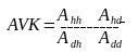
-Ahh corresponds to the sensitivity of the retrieved humidity profile to real variations of humidity
-Add corresponds to the sensitivity of the retrieved HDO profile to real variations of HDO
-Ahd corresponds to the sensitivity of the retrieved humidity profile to real variations of HDO
-Adh corresponds to the sensitivity of the retrieved HDO profile to real variations of humidity
The corresponding δD profile is computed from variables hdo_bc_profiles and h2o_profiles:
Averaging kernels type 2
As there is more vertical information in the retrieved profile of humidity than HDO, there is a difference in vertical sensitivity between the humidity and δD profiles.
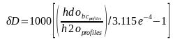
For this reason, Wiegele et al., introduced a methodology to a posteriori correct the difference of vertical sensitivities in order to ensure that both humidity profile and δD profile are representative of the exact atmosphere. This a posteriori correction is provided in the netcdf files. When considering this approach, variables Aaa,
h2o_t2 and dd_t2 must be used. The humidity profiles have been degraded to the vertical sensitivity of δD and Aaa (same structure than AVK) describe this sensitivity. The sub-blocks Ahh and Add are in that case identical.
For simplicity it is recommended to use this type 2 product.
Error analysis 2: considering the retrieval as an estimate of the true state smoothed by the averaging kernels
This is the ideal approach. In comparisons model – data, this approach should be used. The error to consider in that case is the error due to uncertainties in model parameters (2) and the error due to the measurement noise (3). The resulting error has been estimated to 38 permil (between 3 and 6 km) on an individual basis. When considering several
measurements, this error which is random can be reduced by a factor sqrt(n) with n being the number of measurements used in the averaging.
To compare model to data using this approach it is necessary to degrade the vertical information contained in model profiles to the limited sensitivity of the retrieval. This can be easily achieved with the averaging kernels matrix:
For the humidity profile:
First the model profiles need to be interpolated at IASI vertical grid. Then the interpolated q (humidity) profile can be smoothed:
qsm=smoothed profile of q, Ahh=Averaging kernels corresponding to the retrieval of humidity (AVK(1:13,1:13)), q=model humidity profile interpolated at the retrieval levels, In= identity matrix, qp= a priori specific humidity profile used in the retrieval.
The same approach applies for an optimal use of humidity and δD profiles (type 2). In that case, the matrix Aaa must be used.
Error analysis 1: considering the retrieval as an estimate of the true state with an error contribution due to smoothing
If δD retrievals are used in other context that model-data comparison or when the smoothing is not possible, it is important to keep in mind the limited information contained in the retrieved profile. For example, if δD observations at 3.5 km are used
in parallel to airmass trajectory analysis it is important to consider the trajectory of the airmasses arriving between 2 and 5 km and not only at 3.5 km.
Schneider, M., Wiegele, A., Barthlott, S., González, Y., Christner, E., Dyroff, C., García, O. E., Hase, F., Blumenstock, T., Sepúlveda, E., Mengistu Tsidu, G., Takele Kenea, S., Rodríguez, S., and Andrey, J.: Accomplishments of the MUSICA project to provide accurate, long-term, global and high-resolution observations of tropospheric {H2O,δD} pairs – a review, Atmos. Meas. Tech., 9, 2845-2875, https://doi.org/10.5194/amt-9-2845-2016, 2016.
Wiegele, A., Schneider, M., Hase, F., Barthlott, S., García, O. E., Sepúlveda, E., González, Y., Blumenstock, T., Raffalski, U., Gisi, M., and Kohlhepp, R.: The MUSICA MetOp/IASI H2O and δD products: characterisation and long-term comparison to NDACC/FTIR data,
Atmos. Meas. Tech., 7, 2719-2732, https://doi.org/10.5194/amt-7-2719-2014, 2014.
|
|